First of all, it is not a secret that we write this blog as a portfolio for skills that we have been sharpening. We understand the severity of this dataset, and we don’t want to just promote ourselves without respecting all these lives that were lost during the past few months. Having said that, we hope our analysis can be useful for someone or shed some light on some topic not covered yet.
Because not all countries test new cases as it would be necessary, our main focus will be on the number of deaths, and again we would like to highlight our profound respect for all these human lives.
The dataset
In this study we choose the dataset Coronavirus Source Data by Hannah Ritchie. It contains information about new cases, new deaths, and other trends per country and per day. Furthermore it has a few demographic and social indicators per country.
We can download this dataset using the following code:
1
2
3
4
5
6
7
8
9
10
11
12
13
14
15
16
17
18
19
20
21
22
23
24
25
26
27
28
from os import path, makedirs
from urllib import request

import pandas as pd


LOCAL_DIR = 'dataset-covid'
LOCAL_FILE = path.join(LOCAL_DIR, 'owid-covid-data.csv')
REMOTE_URL = 'https://covid.ourworldindata.org/data/owid-covid-data.csv'


def load_covid_data(refresh: bool = False) -> pd.DataFrame:
    if refresh:
        makedirs(LOCAL_DIR, exist_ok=True)
        request.urlretrieve(REMOTE_URL, LOCAL_FILE)

    temp = pd.read_csv(LOCAL_FILE)
    temp = temp[(~temp['iso_code'].isna()) & (~temp['continent'].isna())]
    temp['date'] = pd.to_datetime(temp['date'])

    boundary_dates = temp.groupby('iso_code')['date'].agg([min, max]).reset_index()
    boundary_dates.columns = ['iso_code', 'min_date', 'max_date']
    temp = pd.merge(temp, boundary_dates, on='iso_code', how='left')

    temp.index = temp['date']
    return temp

dataset_covid = load_covid_data()
Random walk model
For a given country, the total number of deaths $D_n$ up until a certain day $n = 0, 1, 2, \dots$ is equal to the sum of the daily deaths $d_0 + d_1 + \dots + d_n$. Our end goal is to find a time dependent probability distribution $P(d, t)$ that we can use to estimate the number of deaths at any time $t$.
There is an assumption here that all daily deaths $d_i$ are drawn from the same probability distribution function. Our fist task is to find this probability distribution function $P(d)$ for each country.
We start by looking at the histograms of daily deaths for a few countries.
1
2
3
4
5
6
7
8
9
10
11
12
13
14
15
16
17
18
19
20
21
22
23
24
25
26
27
28
29
import matplotlib.pyplot as plt
import pandas as pd
import seaborn as sns
sns.set(style="darkgrid")


def worst_country(continent_df: pd.DataFrame) -> str:
    return continent_df.sort_values(by='total_cases',
                                    ascending=False)['iso_code'].values[0]

worst_countries = dataset_covid.groupby('continent').agg(worst_country)['total_cases']
covid_sample = dataset_covid[dataset_covid['iso_code'].isin(worst_countries)]

fig, axs = plt.subplots(2, 3, figsize=(16, 10))

metric = 'new_deaths'
countries = worst_countries.to_dict().items()

for i, (continent, country) in enumerate(countries):
    ax = axs[i // 3][i % 3]
    data = covid_sample[covid_sample['iso_code'] == country][metric]
    sns.distplot(data, label=country, ax=ax)
    ax.legend()
    ax.set_xlabel('Daily deaths')
    ax.set_ylabel('Daily deaths PDF')

# plt.show()
fig.tight_layout()
plt.show()
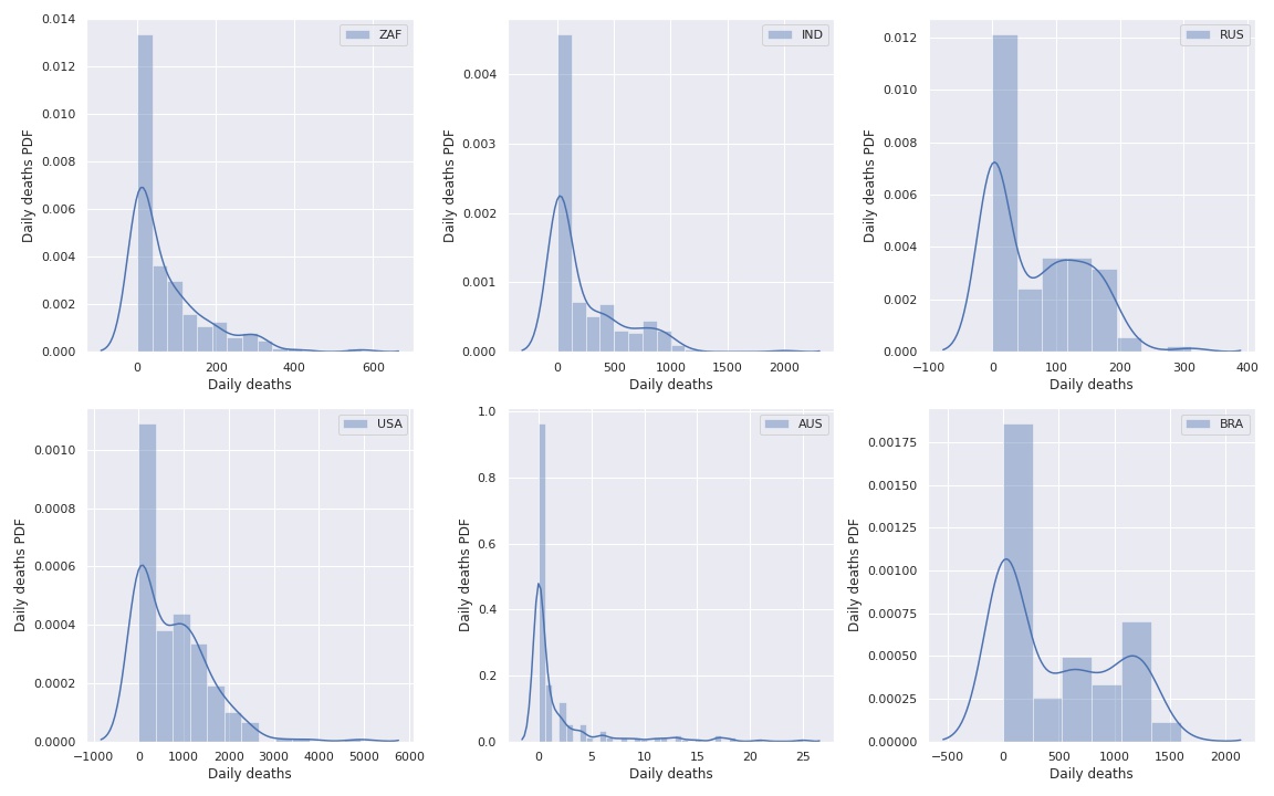
The problem with these histograms is that not all countries start in the beginning of the time series. We can see that in the following image.
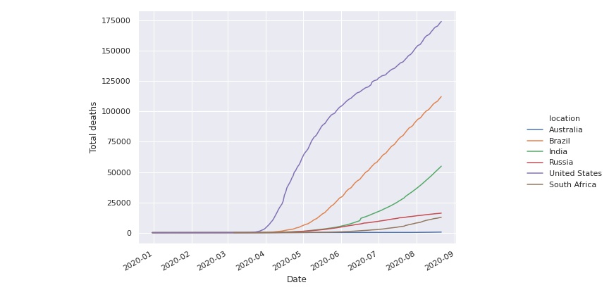
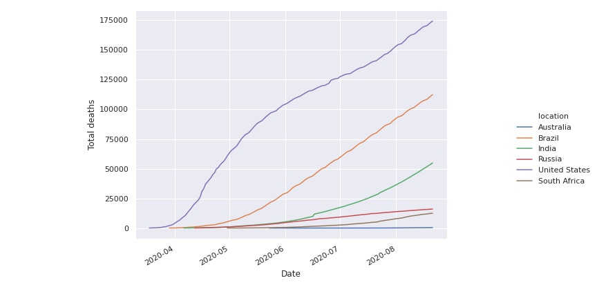
We can remove this transient effect in the beginning by removing days until the total number of deaths is greater than a certain threshold, for instance one hundred.
1
2
3
4
5
6
7
8
9
data_100 = covid_sample[(covid_sample['total_deaths'] > 100)]

g = sns.relplot(ci=None, x='date', y='total_deaths',
                hue='location', kind='line', data=data_100)
g.fig.set_figwidth(12)
g.fig.set_figheight(6)
g.fig.autofmt_xdate()
g.set(xlabel='Date', ylabel='Total deaths')
plt.show()
Then we plot again the histograms
1
2
3
4
5
6
7
8
9
10
11
12
13
14
15
16
17
18
sns.set(style="darkgrid")

fig, axs = plt.subplots(2, 3, figsize=(16, 10))

metric = 'new_deaths'
countries = worst_countries.to_dict().items()

for i, (continent, country) in enumerate(countries):
    ax = axs[i // 3][i % 3]
    data = data_100[data_100['iso_code'] == country][metric]
    sns.distplot(data, label=country, ax=ax)
    ax.legend()
    ax.set_xlabel('Daily deaths')
    ax.set_ylabel('Daily deaths PDF')

# plt.show()
fig.tight_layout()
plt.show()
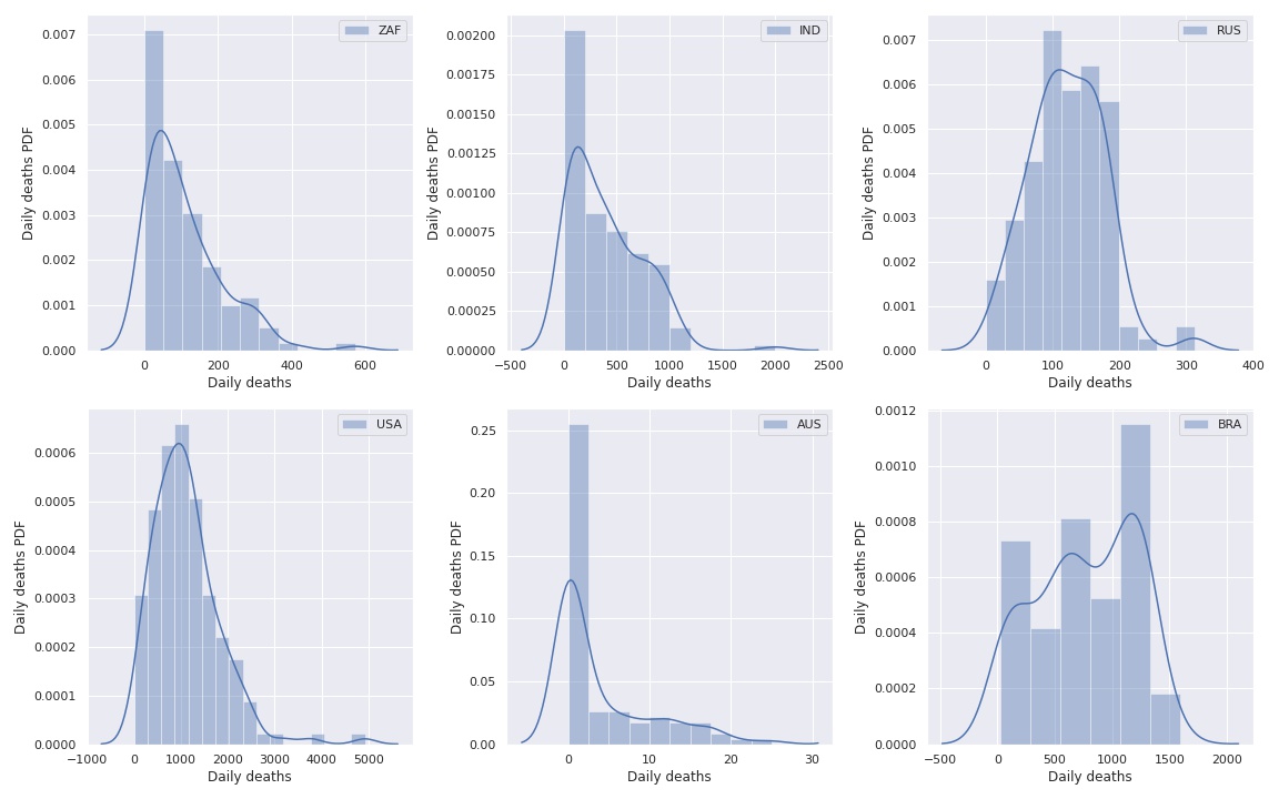
But these distributions are too complex, we need something simpler.
1
2
3
4
5
6
7
8
9
10
11
12
13
14
15
16
17
18
19
20
21
22
23
24
25
26
27
28
29
30
31
32
33
34
35
36
37
38
39
40
41
42
43
44
45
46
47
48
49
50
51
52
53
54
import numpy as np
import scipy.stats as st


fig, axs = plt.subplots(2, 3, figsize=(16, 10))


def get_histogram_dist(data):
    hist, bin_edges = np.histogram(data, density=True)
    hist_centers = [
        (bin_edges[i] + bin_edges[i+1]) / 2
        for i in range(len(bin_edges) - 1)
    ]
    width = 0.1 * (max(hist_centers) - min(hist_centers))
    return hist_centers, hist, width


def get_best_dist(data):
    d = np.linspace(0, data.max(), 1000)

    dist_results = []
    dist_params = {}

    for dist_name in ['lognorm', 'lomax', 'norm', 'skewnorm']:
        dist = getattr(st, dist_name)
        params = dist.fit(data)
        dist_params[dist_name] = params
        # Kolmogorov-Smirnov test
        _, p = st.kstest(data, dist_name, args=params)
        dist_results.append((dist_name, p))

    best_dist, _ = (max(dist_results, key=lambda item: item[1]))
    params = dist_params[best_dist]
    return d, getattr(st, best_dist).pdf(d, *params)


metric = 'new_deaths'
countries = worst_countries.to_dict().items()

for i, (continent, country) in enumerate(countries):
    ax = axs[i // 3][i % 3]

    country_data = data_100[data_100['iso_code'] == country][metric].values
    hist_centers, hist, width = get_histogram_dist(country_data)
    d, d_dist = get_best_dist(country_data)

    ax.bar(hist_centers, hist, width=width)
    ax.plot(d, d_dist, color='orange', linewidth=3, label=country)

    ax.legend()
    ax.set_xlabel('Daily deaths')
    ax.set_ylabel('Daily deaths PDF')

plt.show()
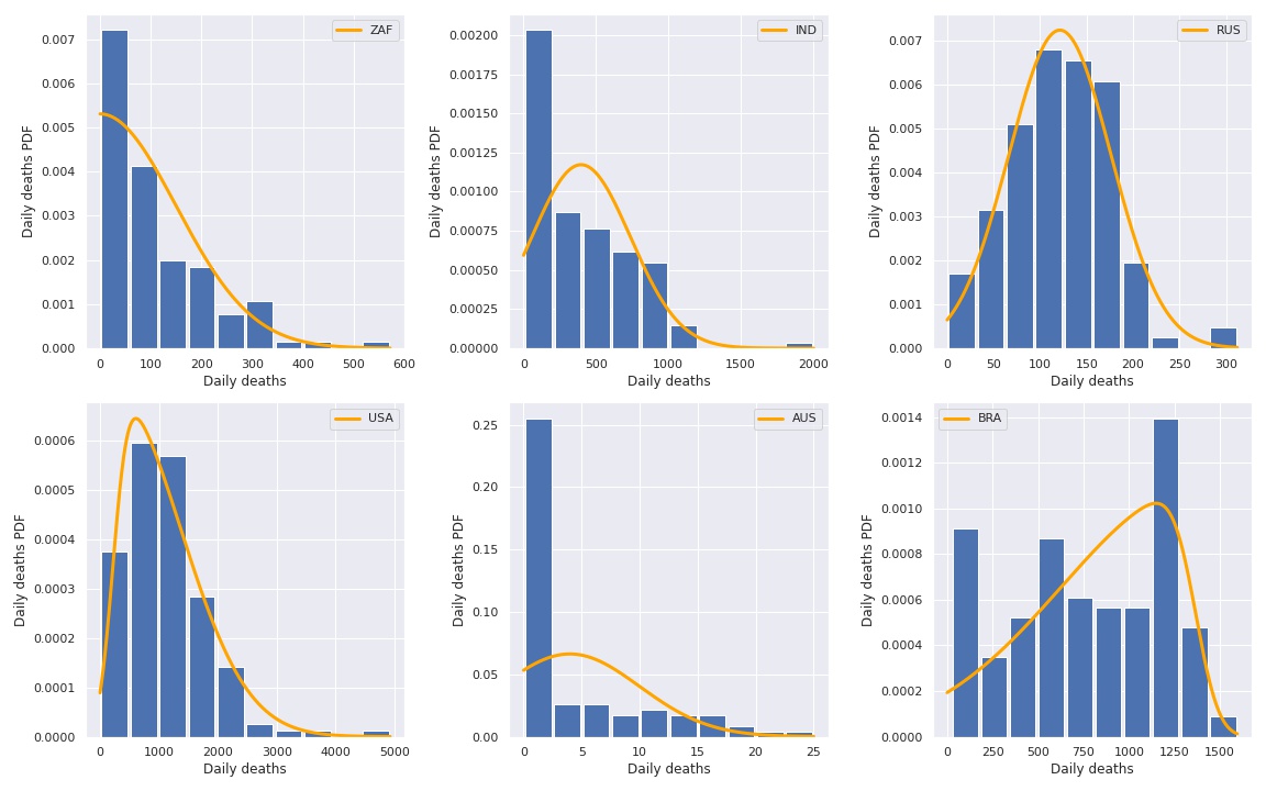
Once we have the distributions $P(d)$, we need to calculate the characteristic function. It defined as the Fourier transform of $P(d)$.
\[g(k) = \int P(d) \mathrm{e}^{i k d}\,\mathrm{d}d\]Using this function, we can obtain the time dependent probability distribution $P(d, t)$ using the following equation:
\[P(d, t) = \frac{1}{2 \pi} \int {g(k)}^{t / 2 \pi \Delta d} \mathrm{e}^{-i k d}\,\mathrm{d}k\]Which means, we take the $g(k)$ to the power $t / 2 \pi \Delta d$ and perform the inverse Fourier transform. The number $\Delta d$ is the precision of the grid of $d$.
The following code executes the procedure described above.
1
2
3
4
5
6
7
8
9
10
11
12
13
14
15
16
17
18
19
20
21
22
23
24
25
26
27
28
29
30
31
32
33
34
35
36
37
38
39
40
41
42
43
44
45
46
47
48
49
50
51
52
53
54
55
56
57
58
59
60
61
62
63
64
65
66
67
68
69
70
71
72
from scipy import fft
from scipy.integrate import simps


def get_best_distribution_(data):
    dist_results = []
    dist_params = {}

    for dist_name in ['lognorm', 'norm', 'skewnorm']:
        dist = getattr(st, dist_name)
        params = dist.fit(data)
        dist_params[dist_name] = params
        # Kolmogorov-Smirnov test
        _, p = st.kstest(data, dist_name, args=params)
        dist_results.append((dist_name, p))

    best_dist, _ = (max(dist_results, key=lambda item: item[1]))
    params = dist_params[best_dist]
    return best_dist, params


def scale_pdf_to_one(pdf, x):
    a = simps(pdf, x)
    return pdf / a


def rho(d, t, dist_name, params):
    dd = 1.0 / (2 * np.pi * (d[1] - d[0]))

    dist = getattr(st, dist_name).pdf(d, *params)
    dist = scale_pdf_to_one(dist, d)

    gk = fft.fft(dist)

    Gk = gk ** (t * dd)

    rho_ = fft.ifft(Gk).real

    return scale_pdf_to_one(rho_, d)


fig, axs = plt.subplots(2, 3, figsize=(16, 10))
for i, (continent, country) in enumerate(countries):
    country_data = data_100[data_100['iso_code'] == country][metric].values
    total_deaths = data_100[data_100['iso_code'] == country][metric].cumsum()
    timeline = np.arange(0, total_deaths.size)

    best_dist, params = get_best_distribution_(country_data)

    if len(params) == 3:
        a, loc, scale = params
    else:
        loc, scale = params

    d = np.linspace(0, loc + 3 * scale, 2 * int(country_data.size))
    dd = d[1] - d[0]

    expected = []
    for t_ in timeline[1:]:
        expected.append(simps(d * rho(d, t_, best_dist, params), d, dd))

    ax = axs[i // 3][i % 3]

    ax.plot(timeline[1:], np.cumsum(expected), label='random walk')
    ax.plot(timeline, total_deaths, label='total deaths')
    ax.set_title(country)
    ax.set_ylabel('Total deaths')
    ax.set_xlabel('Days since threshold')
    ax.legend()

plt.tight_layout()
plt.show()
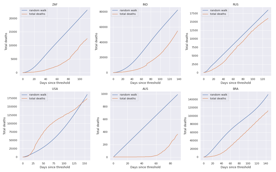
And the result is:
Conclusion
The random walk extrapolation seems to be appropriate when the Maximum Likelihood Estimate fits well the number of daily deaths.
References
- Dinâmica Estocástica e Irreversibilidade. Tânia Tomé, Mário José de Oliveira. 2. ed. rev. e ampl. São Paulo: Editora da Universidade de São Paulo, 2014. ISBN 978-85-314-1480-0.