In this post we will try to use some ensemble methods to deal with an image classification problem. It is not the best application for these methods, but we can still find interesting results. Actually, as we will see, despite of the low capacity of the models to capture the complexity of the problem, they perform almost as good as a human would ;)
The data set
The Fashion Mnist data set is available on Kaggle.
If we download and extract it into a directory named dataset, we should see this structure:
$ tree dataset/
dataset/
├── fashion-mnist_test.csv
├── fashion-mnist_train.csv
├── t10k-images-idx3-ubyte
├── t10k-labels-idx1-ubyte
├── train-images-idx3-ubyte
└── train-labels-idx1-ubyte

0 directories, 6 files
In those two csv files, each line containers the label in the first columns, and it is followed by 748 columns, each on containing one pixel.
We can use the following code to load the training and test sets.
1
2
3
4
5
6
7
8
9
10
import numpy as np
import pandas as pd

def load_images(filename: str):
    images = pd.read_csv(filename)
    return (images.iloc[:, 1:].values.astype(np.uint8),
            images.iloc[:, 0].values.astype(np.uint8))

X_train, y_train = load_images('dataset/fashion-mnist_train.csv')
X_test, y_test = load_images('dataset/fashion-mnist_test.csv')
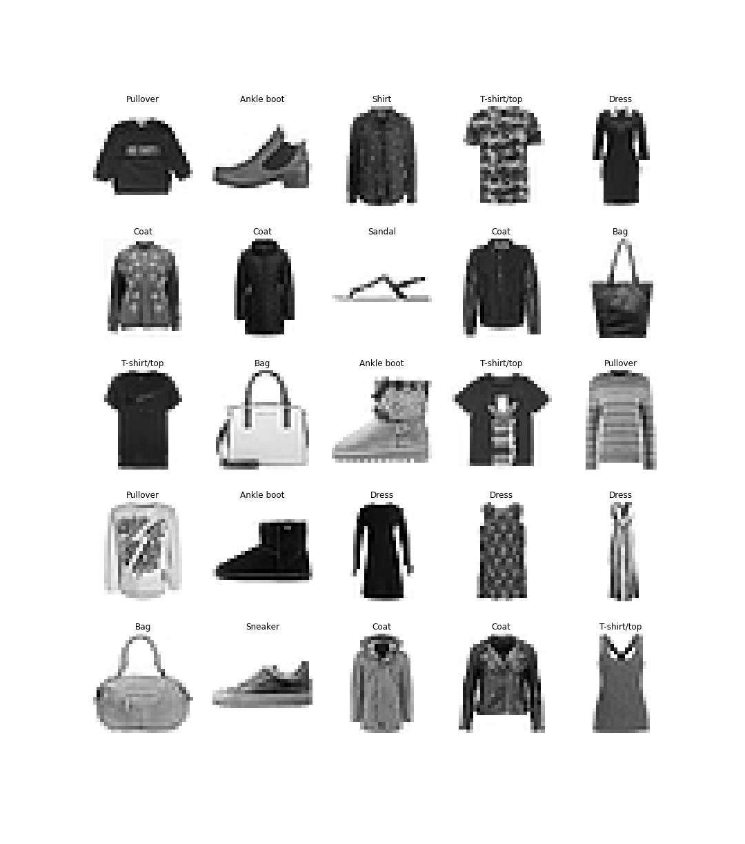
And we can use the following code to visualize the first 25 images.
1
2
3
4
5
6
7
8
9
10
11
12
13
14
15
16
17
18
import matplotlib.pyplot as plt

classes = ['T-shirt/top', 'Trouser', 'Pullover',
           'Dress', 'Coat', 'Sandal', 'Shirt',
           'Sneaker', 'Bag', 'Ankle boot']

fig, ax = plt.subplots(5, 5, figsize=(15, 17))

for i in range(5):
    for j in range(5):
        image = X_train[i * 5 + j]
        label = y_train[i * 5 + j]
        ax[i][j].imshow(image.reshape(28, 28),
                        cmap='binary')
        ax[i][j].set_title(classes[label])
        ax[i][j].axis('off')

plt.show()
The result should look like this:
Pre-processing
The will be no heavy pre-processing here other than a MinMaxScaler. Since the images are encoded as pixels ranging from 0 to 255, adjusting to the range [0, 1] will allow us to test a wider variety of estimators.
Training a model
We can start testing how a Logistic Regression performs when reading pixels only.
1
2
3
4
5
6
7
8
9
10
11
12
13
14
from sklearn.linear_model import LogisticRegression
from sklearn.metrics import classification_report
from sklearn.model_selection import cross_val_predict
from sklearn.pipeline import Pipeline
from sklearn.preprocessing import MinMaxScaler


pipe_lr = Pipeline([
    ('scaler', MinMaxScaler()),
    ('lg_clf', LogisticRegression(multi_class='ovr'))
])

y_pred_lr = cross_val_predict(pipe_lr, X_train, y_train,
                              cv=5, n_jobs=-1, verbose=2)
Which leads to:
>>> print(classification_report(y_train, y_pred_lr,
                                digits=4, target_names=classes))

              precision    recall  f1-score   support

 T-shirt/top     0.7899    0.8277    0.8083      6000
     Trouser     0.9746    0.9650    0.9698      6000
    Pullover     0.7529    0.7612    0.7570      6000
       Dress     0.8391    0.8758    0.8570      6000
        Coat     0.7462    0.7815    0.7634      6000
      Sandal     0.9396    0.9312    0.9354      6000
       Shirt     0.6671    0.5648    0.6117      6000
     Sneaker     0.9196    0.9323    0.9259      6000
         Bag     0.9319    0.9437    0.9377      6000
  Ankle boot     0.9508    0.9467    0.9487      6000

    accuracy                         0.8530     60000
   macro avg     0.8512    0.8530    0.8515     60000
weighted avg     0.8512    0.8530    0.8515     60000
The result is of course not even close to one that we could obtain using a CNN, but it also says we can have some fun here, after all, randomly we should expect less than 10% of accuracy (there are 9 classes).
If we try something a little bit more ambitious:
1
2
3
4
5
6
7
8
9
10
from sklearn.ensemble import RandomForestClassifier


pipe_rf = Pipeline([
    ('scaler', MinMaxScaler()),
    ('rf_clf', RandomForestClassifier())
])

y_pred_rf = cross_val_predict(pipe_rf, X_train, y_train,
                              cv=5, n_jobs=-1, verbose=2)
We already get 2.73% in the f1 score.
>>> print(classification_report(y_train, y_pred_rf,
                                digits=4, target_names=classes))

              precision    recall  f1-score   support

 T-shirt/top     0.8219    0.8620    0.8415      6000
     Trouser     0.9930    0.9637    0.9781      6000
    Pullover     0.7828    0.8170    0.7995      6000
       Dress     0.8739    0.9158    0.8944      6000
        Coat     0.7741    0.8312    0.8016      6000
      Sandal     0.9681    0.9607    0.9644      6000
       Shirt     0.7393    0.5932    0.6582      6000
     Sneaker     0.9362    0.9362    0.9362      6000
         Bag     0.9586    0.9715    0.9650      6000
  Ankle boot     0.9457    0.9525    0.9491      6000

    accuracy                         0.8804     60000
   macro avg     0.8794    0.8804    0.8788     60000
weighted avg     0.8794    0.8804    0.8788     60000
The two estimators together are not better than the RandomForestClassifier.
1
2
3
4
5
6
7
8
9
10
11
12
13
14
from sklearn.ensemble import VotingClassifier


pipe_vote = Pipeline([
    ('scaler', MinMaxScaler()),
    ('voting_clf', VotingClassifier(
        estimators=[
            ('lr', LogisticRegression(multi_class='ovr')),
            ('rf', RandomForestClassifier())
        ], voting='soft', n_jobs=-1))
])

y_pred_voting = cross_val_predict(pipe_vote, X_train, y_train,
                                  cv=5, n_jobs=-1, verbose=2)
>>> print(classification_report(y_train, y_pred_voting,
                                digits=4, target_names=classes))

              precision    recall  f1-score   support

 T-shirt/top     0.8055    0.8633    0.8334      6000
     Trouser     0.9864    0.9690    0.9776      6000
    Pullover     0.7845    0.7992    0.7918      6000
       Dress     0.8695    0.9052    0.8870      6000
        Coat     0.7701    0.8242    0.7962      6000
      Sandal     0.9641    0.9525    0.9582      6000
       Shirt     0.7256    0.5818    0.6458      6000
     Sneaker     0.9330    0.9445    0.9387      6000
         Bag     0.9495    0.9628    0.9561      6000
  Ankle boot     0.9552    0.9550    0.9551      6000

    accuracy                         0.8758     60000
   macro avg     0.8743    0.8757    0.8740     60000
weighted avg     0.8743    0.8758    0.8740     60000
What about 5 LogisticRegression estimators together with a RandomForestClassifier one?
1
2
3
4
5
6
7
8
9
10
11
12
13
14
15
from sklearn.ensemble import BaggingClassifier


pipe_vote = Pipeline([
    ('scaler', MinMaxScaler()),
    ('voting_clf', VotingClassifier(
        estimators=[
            ('lr', BaggingClassifier(LogisticRegression(multi_class='ovr'),
                                     n_estimators=5)),
            ('rf', RandomForestClassifier())
        ], voting='soft', n_jobs=-1))
])

y_pred_voting = cross_val_predict(pipe_vote, X_train, y_train,
                                  cv=5, n_jobs=-1, verbose=2)
>>> print(classification_report(y_train, y_pred_voting,
                                digits=4, target_names=classes))

              precision    recall  f1-score   support

 T-shirt/top     0.8094    0.8613    0.8346      6000
     Trouser     0.9869    0.9680    0.9774      6000
    Pullover     0.7797    0.7953    0.7875      6000
       Dress     0.8673    0.9063    0.8864      6000
        Coat     0.7700    0.8212    0.7947      6000
      Sandal     0.9646    0.9533    0.9589      6000
       Shirt     0.7229    0.5862    0.6474      6000
     Sneaker     0.9343    0.9452    0.9397      6000
         Bag     0.9519    0.9628    0.9573      6000
  Ankle boot     0.9544    0.9555    0.9549      6000

    accuracy                         0.8755     60000
   macro avg     0.8741    0.8755    0.8739     60000
weighted avg     0.8741    0.8755    0.8739     60000
What is going here is that ensemble learning only works when we can trade more bias for lower variance. However, our models are not capable of capturing the high complexity of the task in hand, which means, our bias is already very high, so we have nothing to trade.
There are two ways out of this situation:
- We simplify the task.
- We increase the model’s capacity.
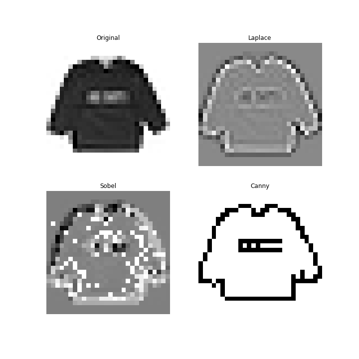
Let’s try yo make the problem simpler. One idea is to replace pictures with their edges. There are a few ways of doing this, and OpenCV is the perfect tool for that.
The following code shows a few edge detection techniques:
1
2
3
4
5
6
7
8
9
10
11
12
13
14
15
16
17
18
19
20
21
22
23
24
25
26
27
28
29
30
31
32
33
import cv2


plt.figure(figsize=(10, 10))

original = X_train[0].reshape(28, 28)

plt.subplot(221)
plt.imshow(original, cmap='binary')
plt.title('Original')
plt.axis('off')

laplace = cv2.Laplacian(original, cv2.CV_64F)
plt.subplot(222)
plt.imshow(laplace, cmap='binary')
plt.title('Laplace')
plt.axis('off')

sobel_x = cv2.Sobel(original, cv2.CV_64F, 0, 1, ksize=1)
sobel_y = cv2.Sobel(original, cv2.CV_64F, 1, 0, ksize=1)
sobel = cv2.bitwise_or(sobel_x, sobel_y)
plt.subplot(223)
plt.imshow(sobel, cmap='binary')
plt.title('Sobel')
plt.axis('off')

canny = cv2.Canny(original, 20, 170)
plt.subplot(224)
plt.imshow(canny, cmap='binary')
plt.title('Canny')
plt.axis('off')

plt.show()
And the result we can see in the next image:
In order to test whether applying edge detection is a good idea, we can create an EdgeDetector transformer.
1
2
3
4
5
6
7
8
9
10
11
12
13
14
15
16
17
18
19
20
21
22
23
24
25
26
27
28
29
30
31
32
33
from sklearn.base import BaseEstimator, TransformerMixin


class EdgeDetector(BaseEstimator, TransformerMixin):
    def __init__(self, edge_technique: str = 'canny'):
        assert edge_technique in ('canny', 'laplace',
                                  'original', 'sobel')
        self.edge_technique = edge_technique

    def fit(self, X, y=None):
        return self

    def transform(self, X):
        X_adj = np.zeros(X.shape)

        for i in range(X.shape[0]):
            original = X[i].reshape(28, 28)

            if self.edge_technique == 'canny':
                edged = cv2.Canny(original, 20, 170)
            elif self.edge_technique == 'laplace':
                edged = cv2.Laplacian(original, cv2.CV_64F)
            elif self.edge_technique == 'sobel':
                sobel_x = cv2.Sobel(original, cv2.CV_64F, 0, 1, ksize=3)
                sobel_y = cv2.Sobel(original, cv2.CV_64F, 1, 0, ksize=3)
                sobel = cv2.bitwise_or(sobel_x, sobel_y)
                edged = np.nan_to_num(sobel, nan=0.0, posinf=0, neginf=0)
            else:
                edge = original

            X_adj[i] = edged.reshape(784)

        return X_adj
And then we can use GridSearchCV to test which one is the best option:
1
2
3
4
5
6
7
8
9
10
11
12
13
14
15
16
17
18
from sklearn.model_selection import GridSearchCV


param_grid = [{
    'edge_detector__edge_technique': ['canny', 'laplace',
                                      'original', 'sobel']
}]

pipe_edge = Pipeline([
    ('edge_detector', EdgeDetector()),
    ('scaler', MinMaxScaler()),
    ('rf_clf', RandomForestClassifier())
])

search = GridSearchCV(pipe_edge, param_grid, scoring='f1_weighted',
                      cv=5, verbose=2, n_jobs=-1)

search.fit(X_train, y_train)
And the best technique according to this experiment is the Sobel, which we use to predict the test set.
>>> y_pred = search.best_estimator_.predict(X_test)
>>> print(classification_report(y_test, y_pred,
                                digits=4, target_names=classes))

              precision    recall  f1-score   support

 T-shirt/top     0.8142    0.8500    0.8317      1000
     Trouser     0.9907    0.9620    0.9762      1000
    Pullover     0.7910    0.8100    0.8004      1000
       Dress     0.8680    0.9210    0.8937      1000
        Coat     0.7808    0.8550    0.8162      1000
      Sandal     0.9718    0.9320    0.9515      1000
       Shirt     0.7571    0.5860    0.6607      1000
     Sneaker     0.9243    0.9280    0.9261      1000
         Bag     0.9277    0.9620    0.9445      1000
  Ankle boot     0.9243    0.9530    0.9385      1000

    accuracy                         0.8759     10000
   macro avg     0.8750    0.8759    0.8740     10000
weighted avg     0.8750    0.8759    0.8740     10000
Although we have a model that is generalizing quite well, it is clearly underfitting, because the problem is too complex to be solved pixel-wise.
Let’s have a look in those images that are not being classified properly to check if we can get some insight. For that, we wil use the ExtraTreesClassifier classifier, which is an extreme version of Random Forests, where the threshold used when splitting instances between trees’ nodes is random instead of optimal for reducing Gini or Entropy.
1
2
3
4
5
6
7
8
9
10
11
12
13
14
from sklearn.ensemble import ExtraTreesClassifier
from sklearn.metrics import classification_report
from sklearn.model_selection import cross_val_predict
from sklearn.pipeline import Pipeline
from sklearn.preprocessing import MinMaxScaler


pipe_et = Pipeline([
    ('scaler', MinMaxScaler()),
    ('et_clf', ExtraTreesClassifier())
])

y_pred_et = cross_val_predict(pipe_et, X_train, y_train,
                               cv=5, n_jobs=3, verbose=3)
>>> print(classification_report(y_train, y_pred_et,
                                digits=4, target_names=classes))
              precision    recall  f1-score   support

aT-shirt/top     0.8148    0.8658    0.8395      6000
     Trouser     0.9936    0.9630    0.9781      6000
    Pullover     0.7828    0.8210    0.8014      6000
       Dress     0.8722    0.9190    0.8950      6000
        Coat     0.7789    0.8220    0.7999      6000
      Sandal     0.9694    0.9562    0.9627      6000
       Shirt     0.7378    0.5915    0.6566      6000
     Sneaker     0.9342    0.9435    0.9388      6000
         Bag     0.9635    0.9712    0.9673      6000
  Ankle boot     0.9486    0.9527    0.9506      6000

    accuracy                         0.8806     60000
   macro avg     0.8796    0.8806    0.8790     60000
weighted avg     0.8796    0.8806    0.8790     60000
Now we train our model once again, and separate the wrong predictions.
1
2
3
4
5
6
7
8
9
10
11
12
13
14
15
16
17
18
19
20
21
22
23
24
25
26
27
28
from sklearn.model_selection import train_test_split

X_train_, X_val, y_train_, y_val = \
    train_test_split(X_train, y_train, random_state=42, test_size=0.2)

pipe_et.fit(X_train_, y_train_)
y_pred = pipe_et.predict(X_val)

X_wrong = X_val[y_pred != y_val]
y_wrong = y_val[y_pred != y_val]
y_pred_ = y_pred[y_pred != y_val]

fig, ax = plt.subplots(4, 4, figsize=(10, 12))

wrong_idx = np.random.randint(0, y_wrong.size, 16)

r, w = 0, 0
for i in range(4):
    for j in range(4):
        ax[i][j].set_facecolor('red')
        expected_label = classes[y_wrong[wrong_idx[w]]]
        actual_label = classes[y_pred_[wrong_idx[w]]]
        ax[i][j].set_title(f'{expected_label} - {actual_label}')
        image = X_wrong[wrong_idx[w]]; w += 1
        ax[i][j].imshow(image.reshape(28, 28), cmap='binary')
        ax[i][j].axis('off')

plt.show()
And the result is displayed in the next image. Each title means [expected label] - [predicted label]
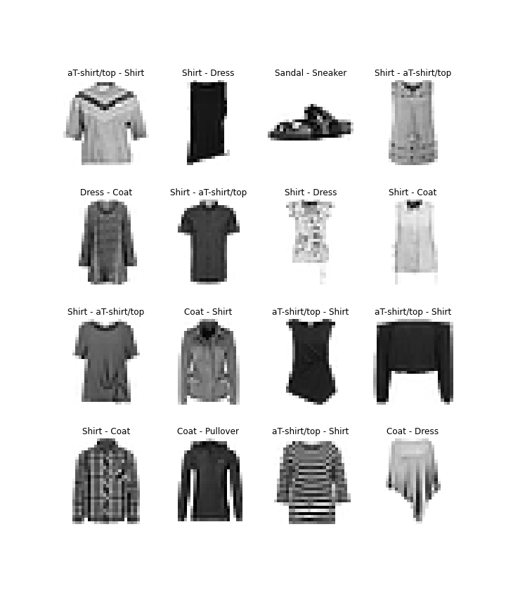
Now we can see that the model fails in images that are really hard to distinguish even for a human.
PCA
Another way to simplify our problem it to use PCA (Principal Component Analysis), in essence, this method finds a lower dimensional space in our data set’s feature space that preserves the data variance as much as possible. Our feature space is currently 784 dimensional, too high. Probably pixels of the edges of the frame are not that important, and maybe others are no important as well.
Using Sciki-Learn’s PCA encoder, we can request to preserve 95% of the data variance using the following code:
1
2
3
4
5
from sklearn.decomposition import PCA


pca = PCA(n_components=0.95)
pca.fit(X_train)
Our training data is a matrix 60000 x 784. The code above computes a matrix N' x 784, where N' is the number of components required in order to keep 95% of the variance (because we asked for 95%). In the transform method, the original data will be multiplied by the transpose of this computed matrix, resulting in a new data set of 60000 x N', where N' < 784. We can check the variance contained in each one of the N' components using the property explained_variance_ratio_.
>>> print(pca.explained_variance_ratio_.shape)
(187, 784)
Which means that 187 pixels positions out of those 784 correspond to 95% of the data set information. Now we are in good shape to test even how a SVM classifier performs in the training set.
1
2
3
4
5
6
7
8
9
10
from sklearn.decomposition import PCA

pipe_svm = Pipeline([
    ('pca', PCA(n_components=0.95)),
    ('scaler', MinMaxScaler()),
    ('svm_clf', SVC())
])

y_pred_svm = cross_val_predict(pipe_svm, X_train, y_train,
                               cv=5, n_jobs=5, verbose=3)
>>> print(classification_report(y_train, y_pred_svm,
                                digits=4, target_names=classes))

              precision    recall  f1-score   support

 T-shirt/top     0.8322    0.8728    0.8520      6000
     Trouser     0.9962    0.9713    0.9836      6000
    Pullover     0.8273    0.8257    0.8265      6000
       Dress     0.8897    0.9207    0.9049      6000
        Coat     0.8306    0.8392    0.8349      6000
      Sandal     0.9570    0.9752    0.9660      6000
       Shirt     0.7500    0.6865    0.7168      6000
     Sneaker     0.9504    0.9618    0.9561      6000
         Bag     0.9707    0.9708    0.9708      6000
  Ankle boot     0.9725    0.9593    0.9659      6000

    accuracy                         0.8983     60000
   macro avg     0.8977    0.8983    0.8977     60000
weighted avg     0.8977    0.8983    0.8977     60000
This result is impressive, it is above TensorFlow’s accuracy for the same problem. The only problem for our argument is that SVM is not an ensemble method.
To address this consistency problem, let’s train a huge VotingClassifier. The reason we changed the MinMaxScaler to the StandardScaler is because it suits better the LogisticRegression model without harming the others.
1
2
3
4
5
6
7
8
9
10
11
12
13
14
15
16
17
18
19
20
21
from sklearn.preprocessing import StandardScaler


pipe_vote = Pipeline([
    ('pca', PCA(n_components=0.95)),
    ('scaler', StandardScaler()),
    ('voting_clf', VotingClassifier(
        estimators=[
            ('lr', BaggingClassifier(LogisticRegression(multi_class='ovr',
                                                        max_iter=1000),
                                     n_estimators=5,
                                     n_jobs=-1)),
            ('svm', BaggingClassifier(SVC(probability=True),
                                      n_estimators=5,
                                      n_jobs=-1)),
            ('rf', RandomForestClassifier()),
            ('erf', ExtraTreesClassifier())
        ], voting='soft', n_jobs=-1))
])

pipe_vote.fit(X_train, y_train)
And the results it:
>>> y_pred = pipe_vote.predict(X_test)
>>> print(classification_report(y_test, y_pred,
                                digits=4, target_names=classes))

              precision    recall  f1-score   support

aT-shirt/top     0.8120    0.8640    0.8372      1000
     Trouser     0.9878    0.9740    0.9809      1000
    Pullover     0.8267    0.8110    0.8188      1000
       Dress     0.8923    0.9200    0.9060      1000
        Coat     0.8276    0.8690    0.8478      1000
      Sandal     0.9673    0.9460    0.9565      1000
       Shirt     0.7446    0.6500    0.6941      1000
     Sneaker     0.9331    0.9350    0.9341      1000
         Bag     0.9568    0.9740    0.9653      1000
  Ankle boot     0.9469    0.9630    0.9549      1000

    accuracy                         0.8906     10000
   macro avg     0.8895    0.8906    0.8895     10000
weighted avg     0.8895    0.8906    0.8895     10000
Conclusion
Applying edge detection was not enough to make the problem simpler, the right way to tackle this problem is using Principal Component Analysis (or PCA).
We saw that dealing with the problem in a pixel-wise manner allows for some interesting predictions.
References
- Hands-On Machine Learning with Scikit-Learn, Keras & TensorFlow, Aurélien Géron (2019). Chapter 7.
- Fashion Mnist, Kaggle (2017).